
Customer Insights
Project Group 33: Sidhant Subramanian, Sreenidhi Reddy Bommu, Bharat Raghunathan, Ayushi Mathur, Vishnu Varma Venkata
Link to Project Presentation: Customer Insights Video
Link to Project Slides: Customer Insights Project Summary
Final
Introduction/Background
Using machine learning (ML) in marketing revolutionises personalised strategies by analysing customer traits. This project aims to harness ML to delve into these traits, enhancing targeted marketing and customer relationships. The untapped potential of ML in extracting and correlating traits from vast datasets offers promising prospects for marketing precision and efficiency.
Using machine learning (ML) in marketing has revolutionised the way businesses approach personalised strategies, fundamentally changing the landscape of customer engagement and relationship management.
By leveraging ML algorithms, marketers can now analyse complex datasets to identify intricate customer traits and preferences that are not immediately apparent., enabling a level of personalization that was previously unattainable.
This capability is particularly valuable in marketing, where understanding the nuances of customer behaviour can lead to more effective and personalised engagement strategies.
Literature Review
Machine learning is crucial for personalized marketing, predicting customer personalities from digital footprints [1], enhancing engagement and sales with personality-tailored advertising [2], and enabling deeper personalization through advanced segmentation techniques based on personality traits [3].
Dataset Description and Link
The Kaggle “Customer Personality Analysis” dataset is used to predict consumer behavior and improve marketing strategies, enhancing business engagement and expenditure optimization.
Dataset Link: Customer Personality Analysis Dataset
Problem and Motivation
Problem
Develop a machine learning model to classify customers based on their likelihood to purchase products from specific categories or channels.
This classification should consider customers’ demographic details (age, education, marital status, income), household composition (number of children and teenagers), engagement history (website visits, recency of purchase), and purchasing behaviour (amount spent on various product categories, number of purchases through different channels, responses to marketing campaigns)
Motivation
The goal is to identify distinct customer segments that prefer different shopping venues (online, in-store, catalog) and product categories (wines, fruits, meats, fish, sweets, gold products), enabling personalized marketing strategies. This model will support targeted marketing initiatives by predicting the preferred shopping channels and product categories for new and existing customers, thereby increasing customer engagement and optimizing marketing spend.
Methods
Data Preprocessing
Feature Correlation
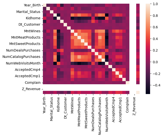
Correlation Plot of all features
Class Distribution
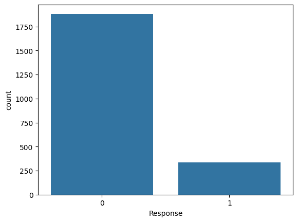
Class Imbalance
Feature encoding
First, each category in a categorical feature was convertedf into a numerical value.
Removing Irrelevant and Highly Correlated Features
The customer ID was dropped since it has no significance in the classification.
Among X variables, highly correlated features(>= 90% correlated with each other) were removed.
Removing Low-Variance Features
Constant features and low-variance features were dropped since they are not useful in our model. Ideally constant features are those with variance = 0. However, to remove both low variance and constant features the threshold was set to 0.01(1.00%)
Standardization
Individual features were standardized by removing the mean and scaling to unit variance to make them conform to a standard normal distribution.
ML Algorithms/Models Implemented
The methodology adopted in this project involved selecting and training supervised learning algorithms to classify customers. Initially, feature selection was applied to identify relevant features and enhance model performance. Following this, supervised learning algorithms such as Random Forest and Linear SVM, were considered for model training. Hyperparameter tuning was then conducted using grid search to optimise the performance of the selected models. Additionally, unsupervised learning technique, K-means clustering, was employed for customer segmentation based on purchasing behaviour. This involved grouping customers into clusters to gain insights for targeted marketing strategies. Overall, the methodology focused on developing accurate and robust classification models to enhance customer segmentation and improve marketing strategies.
Supervised Learning Algorithms
Linear SVM
Linear SVM is a supervised learning algorithm for classification tasks. It separates the data using a single linear decision boundary, making it computationally efficient and effective for high-dimensional datasets. Linear SVM was selected for its simplicity and ability to handle linearly separable datasets. It is particularly useful when dealing with large datasets and is less prone to overfitting compared to more complex models. Additionally, SVMs can handle both linear and non-linear classification tasks through the use of kernel functions, providing flexibility in model selection. Linear SVM can separate the data by a single linear decision boundary, allowing it to effectively classify instances based on their features.
In the implemented solution, hyperparameter tuning was conducted using grid search, a technique aimed at finding the optimal combination of hyperparameters for the Support Vector Machine (SVM) classifier. The hyperparameters tuned include C, gamma, and kernel, which are critical in determining the SVM model’s performance and generalisation capabilities. This process ensures that the SVM model achieves the best possible performance on the given dataset by fine-tuning the parameters to minimise errors and maximise accuracy. Additionally, the simplicity and interpretability of linear SVM make it suitable for understanding the underlying relationships between features and the target variable, providing insights into the classification process.
Random Forest
Random Forest is a powerful ensemble learning method that constructs multiple decision trees during training and outputs the mode of the classes (classification) or the mean prediction (regression) of the individual trees. It was chosen as a supervised learning method due to its versatility, robustness, and effectiveness in handling classification tasks.
Random Forest is well-suited for our project’s objective of classifying customers based on their likely purchase locations. It can handle both numerical and categorical features, is resistant to overfitting, and provides high accuracy even with complex datasets. Additionally, Random Forest can separate the data by non-linear decision boundaries, allowing it to capture intricate patterns in the data that may not be linear in nature.
Moreover, decision trees, the building blocks of Random Forest, inherently consider interactions between variables when making split decisions. This feature enables the algorithm to capture complex relationships and interactions within the data, making Random Forest a versatile and powerful tool for our classification task.
Neural Networks
Neural networks are a class of machine learning algorithms inspired by the structure and function of the human brain. They consist of interconnected nodes, or neurons, organised into layers. In a typical feedforward neural network, information flows from the input layer through one or more hidden layers to the output layer. Each neuron in a layer receives input signals from the neurons in the previous layer, processes them using an activation function, and produces an output signal that is passed to the next layer.
Neural networks are capable of learning complex patterns and relationships within data, making them well-suited for tasks such as classification, regression, and pattern recognition. During the training process, the network adjusts its parameters, or weights, through a process called backpropagation, in order to minimise the difference between its predictions and the true values in the training data.
One of the key advantages of neural networks is their ability to automatically learn hierarchical representations of data, which allows them to capture intricate patterns and dependencies. Additionally, neural networks can generalise well to unseen data, making them robust and suitable for a wide range of applications.
We have developed a Neural Network model due to its ability to model complex patterns and accommodate diverse data distributions. Neural Networks are particularly effective for classifying non-linearly separable data, making them an excellent choice for our dataset, which includes a wide range of customer behaviours and traits. By leveraging deep learning techniques, we aim to uncover intricate relationships within our data that simpler models might miss.
Unsupervised Learning Algorithms
K - Means
K-Means clustering is an unsupervised learning algorithm that partitions data points into clusters based on their similarity. It works by iteratively assigning data points to the nearest cluster centroid and updating the centroids based on the mean of the data points assigned to each cluster. One of the key reasons for selecting K-Means clustering is its ability to work well with datasets of even cluster sizes.
Another advantage of K-Means clustering is its simplicity and interpretability. The algorithm is easy to implement and understand, making it accessible to users with varying levels of expertise in machine learning. By clustering data based on centroids, K-Means provides a clear and intuitive representation of the underlying structure of the data, making it useful for exploratory data analysis and pattern recognition tasks.
In the implemented solution, K-Means clustering was used to group customers based on their purchasing behaviour and identify distinct segments within the dataset. By clustering customers into groups based on their similarity, businesses can gain valuable insights into customer preferences, behaviour, and purchasing patterns. This information can then be used to tailor marketing strategies, improve customer engagement, and drive business growth.
Hierarchical Clustering
Hierarchical clustering is a powerful technique used in exploratory data analysis to uncover underlying structures within a dataset by organising data points into a tree-like hierarchy of clusters. Unlike partition-based methods, hierarchical clustering does not require specifying the number of clusters beforehand, making it particularly useful for datasets where the number of clusters is not known a priori or when exploring the data at different levels of granularity. The algorithm iteratively merges or splits clusters based on their proximity, forming a dendrogram that illustrates the hierarchical relationships between data points.
Hierarchical clustering offers flexibility in choosing distance metrics and linkage methods, allowing customization to suit the specific characteristics of the data. This method provides valuable insights into the inherent structure of the data, aiding in understanding patterns, identifying outliers, and making informed decisions in various domains.
Hierarchical clustering is selected to create a hierarchy of clusters, which can be useful for exploring the structure of the data at different levels of granularity. This model allows us to identify naturally occurring groups within our customer base without pre-specifying the number of clusters.
Hierarchical Clustering is suited for our project as it provides a detailed insight into the customer data’s structure, revealing how customer segments are related at different levels of granularity. It will enable us to develop a detailed understanding of customer preferences and behaviours, helping in coming up with targeted marketing strategies.
OPTICS
The OPTICS (Ordering Points To Identify the Clustering Structure) method is a density-based clustering algorithm that aims to identify clusters of arbitrary shape within a dataset. Unlike traditional clustering algorithms, OPTICS does not require specifying the number of clusters in advance. Instead, it produces a reachability plot, which represents the density-based clustering structure of the data.
OPTICS starts by computing the pairwise distance between all data points and then identifies core points, which are data points with a sufficient number of neighbouring points within a specified distance. By analysing the reachability distance of each point, OPTICS constructs a reachability plot that characterises the density-based structure of the data. This plot allows for the identification of clusters as regions of high density separated by regions of low density.
OPTICS is particularly useful for datasets with varying densities and irregularly shaped clusters, as it can adapt to the local density of the data. Additionally, OPTICS offers parameters such as minimum samples (epsilon), reachability(xi), and minimum cluster size, providing flexibility in adjusting the algorithm’s sensitivity to density variations.
This model helps in handling varying cluster sizes and densities effectively. This model is particularly beneficial for our dataset, which likely contains diverse customer segments. OPTICS helps us identify these segments based on density, overcoming the limitations of models that assume clusters of similar sizes.
By employing OPTICS, we aim to achieve a more flexible and accurate segmentation of our customer base, improving our ability to target marketing efforts effectively.
Results and Discussion
Random Forest
Results:
| Class | Precision | Recall | F1-Score | Support |
|---|---|---|---|---|
| 0 | 0.88 | 0.99 | 0.93 | 567 |
| 1 | 0.77 | 0.24 | 0.37 | 98 |
Accuracy: 87.82%
| Metric | Precision | Recall | F1-Score | Support |
|---|---|---|---|---|
| Macro Avg | 0.83 | 0.62 | 0.65 | 665 |
| Weighted Avg | 0.87 | 0.88 | 0.85 | 665 |
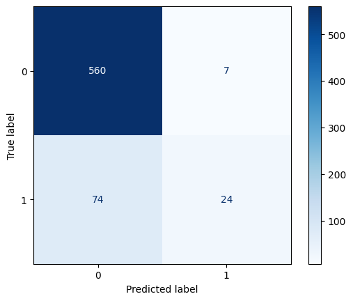
Confusion Matrix for Random Forest
The confusion matrix signifies the effect of the classification model for the given dataset, and random forest perform well for this dataset. We observe that with respect to class 0 the correct predictions highly dominate and perform very well. While for class 1 the number of false predictions dominates. This shows that random forest is not performing effectively for class 1.
Quantitative Metrics
- Precision measures the proportion of true positive predictions among all positive predictions made by the model, it range from 0 to 1. The precision for both classes is well balanced with class 0 being 0.88 and class 1 being 0.77, this implies the local view of the predictions are quite close.
- Recall measures the proportion of true positive instances that were correctly identified by the model, it also ranges from 0 to 1. The recall for class 0 is 0.99 which is very close to 1 and captures the features for class 0 very accurately. However the recall for class 1 is 0.24 which is on the lower side. From the perspective of recall the model predicts very well for class 0 but falls behind for class 1.
- F1 score, which is the harmonic mean of precision and recall. Since we observe that the recall for class 1 is lesser compared to class 0, that impacts the F1 score which captures both precision and recall. The F1 score for class 0 is 0.93 and for class 1 it is 0.37.
- The overall accuracy of the model is 87.82%, the reduction in the accuracy can be attributed to the lower recall for class 1.
SVM
Results:
| Class | Precision | Recall | F1-Score | Support |
|---|---|---|---|---|
| 0 | 0.89 | 0.98 | 0.93 | 567 |
| 1 | 0.70 | 0.27 | 0.39 | 98 |
Accuracy: 87.52%
| Metric | Precision | Recall | F1-Score | Support |
|---|---|---|---|---|
| Macro Avg | 0.79 | 0.62 | 0.66 | 665 |
| Weighted Avg | 0.86 | 0.88 | 0.85 | 665 |
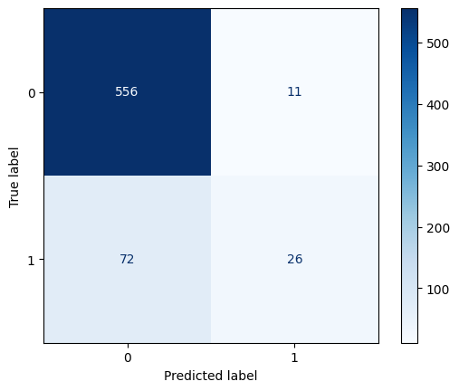
Confusion Matrix for SVM
The confusion matrix signifies the effect of the classification model for the given dataset, and SVM performs well for this dataset. We observe that with respect to class 0 the correct predictions highly dominate and perform very well. While for class 1 the number of false predictions dominates. This shows that the model is not performing effectively for class 1. We shall analyse the models based on quantitative metrics below.
Quantitative Metrics
- We can observe a similar trend for SVM when compared to random forest.
- The precision for both classes is well balanced with class 0 being 0.89 and class 1 being 0.70, this implies the local view of the predictions are quite close.
- The recall for class 0 is 0.98 which is very good, while the recall for class 1 is 0.27 which reduces the metrics such as F1 score and accuracy. From the perspective of recall the model predicts very well for class 0 but falls behind for class 1.
- The trend for F1 score is similar with F1 score for class 0 being 0.93 and for class 1 benign 0.39. In a way when compared with random forest SVM performs slightly better in terms of recall and F1 score.
- The overall accuracy still remains at 87.52%, again the accuracy reduction is attributed to the reduced recall for class 1.
Overall when we look at random forest and SVM the final accuracy is similar but we are concerned with reducing the false negatives or customers who have responded but are classified as customers who have not and since the recall is higher for SVM instead of Random Forest we choose SVM as the better model of the two.
Neural Networks
Results:
| Class | Precision | Recall | F1-Score | Support |
|---|---|---|---|---|
| 0 | 0.90 | 0.96 | 0.93 | 567 |
| 1 | 0.62 | 0.42 | 0.50 | 98 |
Accuracy: 87.67%
| Metric | Precision | Recall | F1-Score | Support |
|---|---|---|---|---|
| Macro Avg | 0.76 | 0.69 | 0.71 | 665 |
| Weighted Avg | 0.86 | 0.88 | 0.87 | 665 |
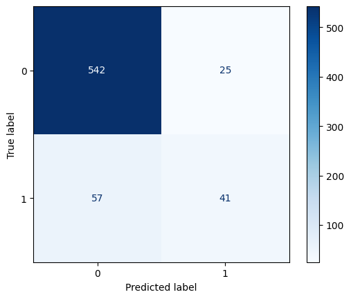
Confusion Matrix for Neural Networks
The confusion matrix signifies the effect of the classification model for the given dataset, and Neural Networks too perform well for this dataset. We observe that with respect to class 0 the correct predictions highly dominate and perform very well. While for class 1 the number of false predictions dominates. This shows that the model is not performing effectively for class 1. We shall analyse the models based on quantitative metrics below.
Quantitative Metrics
- Compared to Random Forests and SVM, Neural Networks have a significant improvement in the F1 Score for class 1 to 0.5, because of the significant improvement in recall to 0.42, which outweighs the decrease in precision.
- This improvement comes at a slight cost, a difference emerges in the precision where it is 0.90 for class 0 but only 0.62 for class 1. The overall recall for class 0 still remains excellent at 0.96.
- The overall accuracy remains at the same range, which is at 87.67%, where the model appears to have traded decreased precision in class 1 for increased recall in class 1.
Summary of Supervised Models
In this problem’s context, the most costly errors are false negatives (FNs) because classifying a customer likely to respond (1) as one who did not (0), can make us lose a potential target/conversion (and thereby revenue), hence this makes the class 1 recall the most important metric. From that perspective, Neural Networks were the best performing model amongst all of them with the highest class 1 recall (0.42) and lowest FNs (57).
K-Means Clustering
Quantitative Metrics
- The silhouette coefficient for the best hyperparameters obtained by grid search is 0.6613. The range of the silhouette coefficient is from -1 to 1. The higher the silhouette coefficient, the better the clustering quality in unsupervised learning. A score close to 1 indicates the data points clustered well and are far away from neighboring clusters. The silhouette coefficient we obtained is close to 1 and signifies that this clustering model is well suited for the given dataset.
Elbow Method
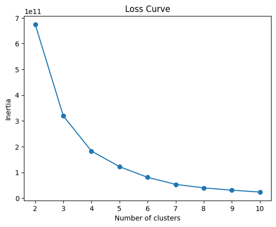
Elbow Method - Inertia
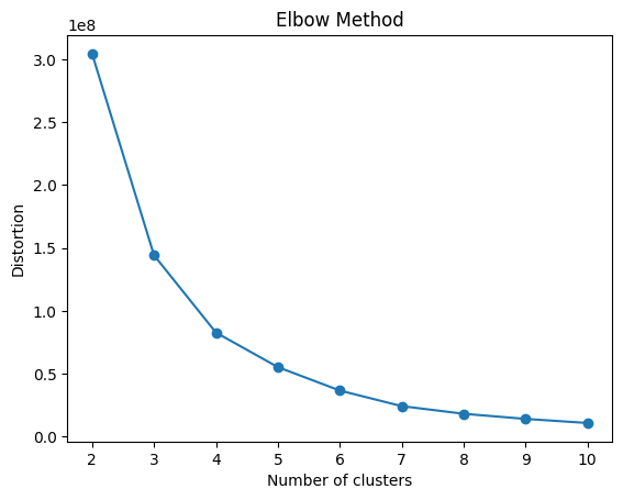
Elbow Method - Distortion
In unsupervised learning and in particular for K-Means, the Elbow method is used to determine the number of clusters. Inertia estimates the sum of squares within the cluster. It measures the squared distances of samples to their closest center. A lower value of inertia is better, implying the clusters are dense and separated.
Distortion measures the average of the squared distances from cluster centers to data points. Lower distortion is better, implying compact clusters and the centroids being close. Both plots can be used to determine the number of clusters.
From the curve, we can determine the number of clusters by identifying the elbow. We can observe that there is a sharp drop in slope after 2 clusters, so the number of clusters can be taken as 2 for the K-means clustering model under consideration, which also matches the best parameter values obtained from hyperparameter grid search.
Hierarchical Clustering
Quantitative Metrics
- In this case, the silhouette coefficient for the best hyperparameters obtained by grid search turns out to be 0.6472. Since a higher silhouette coefficient closer to 1 denotes better clustering quality, we can conclude that hierarchical clustering performs almost at par with K-Means for this dataset.
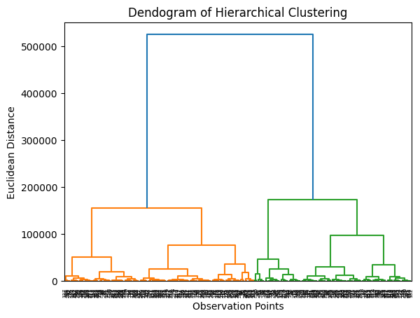
Dendrogram of Hierarchical Clustering
Each branch in a dendrogram represents a cluster and as you move up the tree, clusters are merged into larger clusters. The height at which two branches are joined indicates distance between two clusters, wherein a higher joining point means greater dissimilarity between clusters.
To determine the number of clusters for any given value of distance, a horizontal cut line is made across the tree and the number of vertical lines this intersects is the number of clusters obtained at that value of distance. The distance is typically determined by some criterion specific to the problem. In our case, the largest join height (corresponding to the tall blue lines) corresponds to 2 clusters, hence that appears to be the optimal number of clusters to be considered.
OPTICS
Quantitative Metrics
- For this method, the silhouette coefficient for the best hyperparameters obtained by grid search turns out to be significantly lower at 0.4823. Since a lower silhouette coefficient closer to 0 denotes poorer clustering quality, we can conclude that OPTICS does not perform as well as the previous methods K-Means or Hierarchical Clustering for this dataset.
This could probably mean that the dataset is not split into regions of high density and regions of low density, in other words the data may not be composed of regions of varying densities. Similarly, it could also be due to high-dimensional nature of data, or it could be due to a big difference in cluster sizes.
Supervised Model Analysis
We shall examine the learning curves of all the supervised models trained so far.
Random Forest
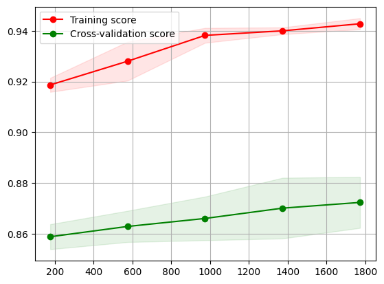
Learning Curve for Random Forest
The learning curve explores the effect of the size of the training data on the training and cross-validation scores. From the learning curve for the random forest, the training score increases profoundly until 1000 samples and beyond that we can see a linear increase as well but not as steep as towards the left half of the plot.
While the cross-validation scores show a trend of increasing testing scores almost linearly throughout as the training sample size is increased. Since both the training and cross-validation scores are increasing and are at a good range of values we don’t observe any overfitting or underfitting in the learning curve.
Considering the right part of the plot where the dataset is large enough, we observe that the training score stands at 0.94 and cross-validation score stands at 0.87. Since both the scores are increasing with higher training sizes it captures the patterns effectively.
SVM
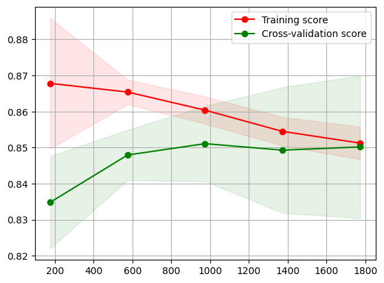
Learning Curve for SVM
For the obtained model after taking the best hyperparameters from cross validation, we have the learning curve. We see that the cross-validation scores increases throughout, even thought the training scores see a slight decrement. This indicates the improvement in generalization of the model as it is improving its ability to generalize to unseen data effectively.
This model captures the underlying patterns of the data that are consistent across different subsets. Since both the training and cross-validation scores are relatively high and the testing scores dont see a decreasing trend we don’t see any overfitting or underfitting in the learning curve.
Overall seeing the trend of training score and cross-validation score it suggests that the model is moving towards a better balance between capturing patterns in the data and generalizing to unseen data.
Neural Networks
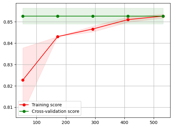
Learning Curve for Neural Network
For this model too, the learning curve is taken on the best hyperparameters found via grid search using cross validation. We can observe that the training scores are increasing (even though cross validation scores remain constant), indicating a well fitted and generalized model.
Since both the training and cross validation scores are at reasonably high values (> 0.8 each), one can infer that the model fitted to the data very quickly and is very gradually improving its generalization capabilities over more iterations.
Observing the overall trend of increasing training scores converging to the high cross validation scores on increasing numbers of samples, the model performance is gradually improving on the training data. However, because the performance is plateauing after a point, adding more data may not significantly improve the model’s performance.
Discussion/Inference
We have built models which can classify whether customers will respond to at least one out of 5 different ad campaigns, and if that is the case, we can send ad campaigns only to that category of customers, thereby focusing resources and reducing overall ad spend.
Unsupervised Cluster Analysis
The plot of the cluster sizes is as follows:
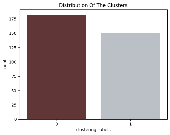
Cluster Distribution
Next, a decision tree was trained (fitted) on the cluster labels in order to examine what features the clusters were composed of.
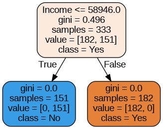
Cluster Features
We find that income is the primary factor for the clustering or in other words, we can infer that the data has been clustered into low-income and high-income groups.
After analyzing all the features, we found significant results in these selected features, wherein the features were compared and contrasted between the two clusters by using boxplots.
Feature: Income
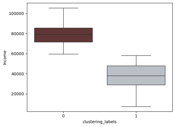
Income Between Clusters
Feature: Amount Spent on Wines
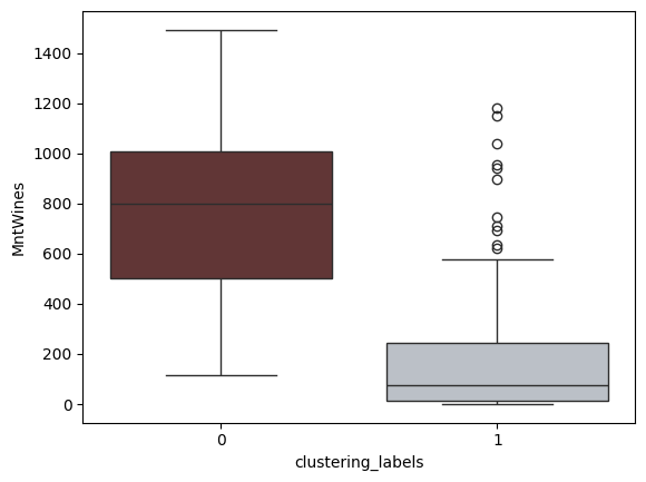
Amount Spent on Wines Between Clusters
Feature: Amount Spent on Meat Products
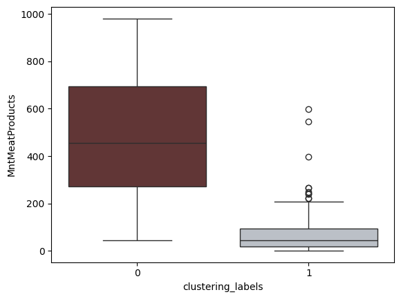
Amount Spent on Meat Products Between Clusters
Feature: Amount Spent on Fish Products
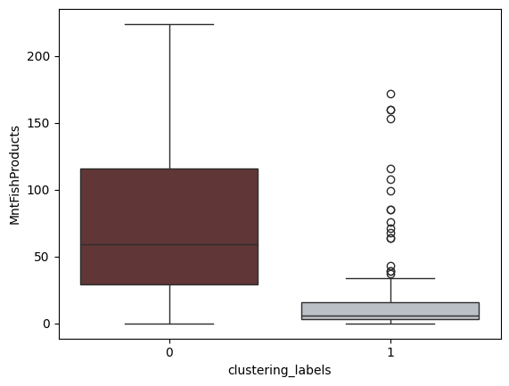
Amount Spent on Fish Products Between Clusters
Discussion/Inference
From these plots, it can be inferred that the clusters are divided into high and low income groups. Additionally, it can be inferred that the high income cluster also spend higher amounts on wines, meat and fish products compared to the lower income cluster. This shall be useful in informing marketers where to target their ad campaigns to cater to such categories of customers.
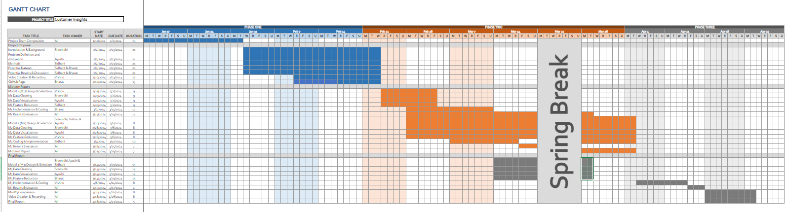
Final Timeline
Link to Gantt Chart Spreadsheet
Contribution Table
| Name | Final Contribution |
|---|---|
| Sreenidhi Reddy Bommu | Data Preprocessing, Presentation |
| Ayushi Mathur | Methods - Supervised and Unsupervised Learning, Next Steps |
| Sidhant Subramanian | Problem Definition, Modeling |
| Bharat Raghunathan | Results and Discussion, GitHub Repository, GitHub Pages |
| Vishnu Varma Venkata | Video, Presentation |
Next Steps
Moving forward, it would be beneficial to further enhance the analysis by considering additional models or methods to gain deeper insights into the dataset. One potential avenue is to explore ensemble clustering techniques, such as Consensus Clustering or Cluster Ensemble, which combine multiple clustering algorithms to improve the robustness and stability of the results. These methods can provide more reliable cluster assignments by aggregating the outputs of individual clustering algorithms.
In these final phases of our customer insights project, the last phase will involve productionizing/deploying existing machine learning models and roll out targeted marketing ads/campaigns based on these models’ performance and our understanding of customer data.
References
[1]: https://doi.org/10.1073/pnas.1218772110 - M. Kosinski, D. Stillwell, and T. Graepel, "Private traits and attributes are predictable from digital records of human behavior," Proceedings of the National Academy of Sciences, vol. 110, no. 15, pp. 5802-5805, April 2013.
[2]: https://www.pnas.org/doi/full/10.1073/pnas.1710966114 - S.C. Matz, M. Kosinski, G. Nave, and D.J. Stillwell, "Psychological targeting as an effective approach to digital mass persuasion," Proceedings of the National Academy of Sciences, vol. 114, no. 48, pp. 12714-12719, November 2017.
[3]: https://doi.org/10.48550/arXiv.2306.17170 - J. Zhang, Y. Wang, and P.S. Yu, "Community structure detection in social networks with node attributes," IEEE Transactions on Knowledge and Data Engineering, vol. 31, no. 10, pp. 1984-1997, Oct. 2019.
[4]: scikit-learn: Machine Learning in Python - F. Pedregosa, G. Varoquaux, A. Gramfort, V. Michel, B. Thirion, O. Grisel, M. Blondel, P. Prettenhofer, R. Weiss, V. Dubourg, J. Vanderplas, A. Passos, D. Cournapeau, M. Brucher, M. Perrot, and E. Duchesnay, "Scikit-learn: Machine Learning in Python," Journal of Machine Learning Research, vol. 12, pp. 2825-2830, 2011.
[5]: Array programming with NumPy - C.R. Harris, K.J. Millman, S.J. van der Walt, R. Gommers, P. Virtanen, D. Cournapeau, E. Wieser, J. Taylor, S. Berg, N.J. Smith, R. Kern, M. Picus, S. Hoyer, M.H. van Kerkwijk, M. Brett, A. Haldane, J. Fernández del Río, M. Wiebe, P. Peterson, P. Gérard-Marchant, K. Sheppard, T. Reddy, W. Weckesser, H. Abbasi, C. Gohlke, T.E. Oliphant, "Array programming with NumPy," Nature, vol. 585, no. 7825, pp. 357-362, Sep. 2020.
[6]: pandas: Pandas - The pandas development team, "pandas-dev/pandas: Pandas," Zenodo, version: latest, Feb. 2020.